Often times, we create a model, add some Conv2D layer there, followed by Maxpooling2D layer, then another Conv2D and Maxpooling2D. Then we trained our model, it overfits our training data, we add some Dropout layer and l2/l1 regularizers. It became somehow resistant to overfitting and our model works better now.
But how can we understand our model more? Only if we can visualize each layer's output.
That would be very helpful I think.
Visualizing Feature Maps
We'll, we can actually visualize each layers output that may guide us on tweaking our model's hyperparameters.
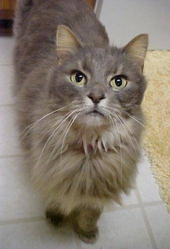
Let's start from loading our sample Image
import tensorflow as tf
from tensorflow.keras.preprocessing import image
import numpy as np

img_path = 'cat.jpg'
img = image.load_img(img_path, target_size=(150, 150))

Load your trained model. It can be any model from your project (Digit Recognizer, Fashion MNIST, etc)
from tensorflow.keras.models import load_model

model = load_model('dogcat_v1.h5')
Here I loaded a simple ConvNet I created previously using Dogs vs Cats datasets.
You can check that blog here.
Let see our model architecture
model.summary()

As you can see, it is a simple network compose of 3 Conv2D layers and 2 MaxPooling2D layers.
Now, let's extract the output of our Conv2D and MaxPooling2D layers and it is located on the first five layers of our model
from tensorflow.keras import models

layer_outputs = [layer.output for layer in model.layers[:5]]
Then create a new multi output model using our original model input.
activation_model = models.Model(inputs=model.input, outputs=layer_outputs)
Note that our original model is a Sequential model that expects only one input data and one output class.
That is usually the case on most classification problem. But some problem may require you to have more than one outputs on your model. For example, on our Dogs vs Cats problem, our task is to classify an Image if it is a Dog or Cat and we create a Sequential model for that.
If our task is to classify if it is a Dog or a Cat and also classify its breed, that's the time we may need a two outputs model.
Using our activation_model, let's try to predict our example image, remember that we convert that image into image tensor.
activations = activation_model.predict(img_tensor)
Let see the shape of the first activation layer
first_layer_activation = activations[0]
print(first_layer_activation.shape)

(1, 148, 148, 16) means, a 148x148 feature map with 16 channels, yours maybe different if you use a different model.
Visualize the first channel
plt.matshow(first_layer_activation[0, :, :,1], cmap='viridis')
plt.show()

Note that it tries to detect the edges of the image but we can still recognize that it is a cat.
Let's try the 3rd channel
plt.matshow(first_layer_activation[0, :, :,3], cmap='viridis')
plt.show()

This looks like a bright green dots detectors that capture the cat's eye and a part of its nose. It is very abstract and given this image, we can hardly guess the original input.
Now let's try to plot every channels on each activation layers
import tensorflow.keras

layer_names = []
for layer in model.layers[:5]:
    layer_names.append(layer.name)

images_per_row = 16

for layer_name, layer_activation in zip(layer_names, activations):

    n_features = layer_activation.shape[-1]

    size = layer_activation.shape[1]

    n_cols = n_features // images_per_row
    display_grid = np.zeros((size * n_cols, images_per_row * size))

    for col in range(n_cols):
        for row in range(images_per_row):
            channel_image = layer_activation[0,
                                             :, :,
                                             col * images_per_row + row]
            # Post-process the feature so we can visualize it
            channel_image -= channel_image.mean()
            channel_image /= channel_image.std()
            channel_image *= 64
            channel_image += 128
            channel_image = np.clip(channel_image, 0, 255).astype('uint8')
            display_grid[col * size : (col + 1) * size,
                         row * size : (row + 1) * size] = channel_image

    if size > 0:
        scale = 1. / size
        plt.figure(figsize=(scale * display_grid.shape[1],
                            scale * display_grid.shape[0]))
        plt.title(layer_name)
        plt.grid(False)
        plt.imshow(display_grid, aspect='auto', cmap='viridis')

plt.show()

Here we can see the magic of ConvNet model. On the first few layers, our model just detects edges, but we can still recognize the input image as cat.
As we move deeper, it became more abstract and we can hardly tell what object is. It detects higher level features like ear, nose, mouth, etc and filtered out all irrelevant information on the image.
Generally, this is the same way on how humans remember when we see object for a few seconds.
We learned the abstract image of it but can't really remember the specifics.
For example, if someone asks you to draw an image of the house you just passed by, you may draw it like this

But this is how the actual house looks like

Thank you for reading this blog. Hope you learn something in this simple tutorial.